SplaTAM: Splat, Track & Map 3D Gaussians for Dense RGB-D SLAM

Summary

SplaTAM: Splat, Track & Map 3D Gaussians for Dense RGB-D SLAM

• 核心: 首次把 3D Gaussian Splatting 作为底层场景表示用于 dense RGB-D SLAM——单一 unposed monocular RGB-D 输入同时估计相机位姿与高保真稠密地图
• 方法: 简化 3DGS（isotropic + view-independent color）→ silhouette-guided differentiable rendering 驱动 tracking / densification / map update 三步在线循环；silhouette 同时作为 tracking gating mask 和 densification trigger
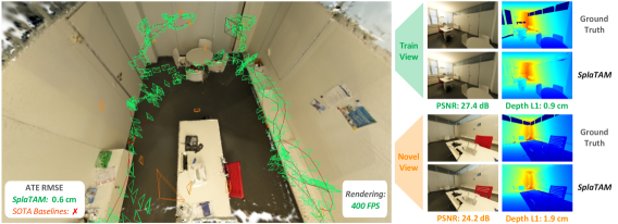
• 结果: Replica ATE 0.36cm（Point-SLAM 0.52）、ScanNet++ 1.2cm（所有 baselines fail）、TUM-RGBD 5.48cm（baselines 8.92）；ScanNet++ novel-view PSNR 24.41 vs Point-SLAM 11.91；rasterization 可达 400 FPS
• Sources: paper | website | github
• Rating: 2 - Frontier（CVPR 2024 早期 3DGS-SLAM 代表作，被后续 3DGS-SLAM 工作普遍作为 baseline；但 SLAM 非我主线研究方向，按 field-centric rubric 定位 Frontier 而非 Foundation）

Key Takeaways:

1. Explicit volumetric beats implicit for SLAM: 3DGS 提供显式空间外延 + 可控容量 + 近线性梯度通路，适合 incremental SLAM；NeRF-style implicit 改一处影响全局、ray sampling 限制效率（Point-SLAM 每 iteration 只采 200-1000 像素，SplaTAM 直接 rasterize 120万像素）
2. Silhouette mask is the trick: 渲染 silhouette $S(\mathbf{p})$ 同时承担两个职责——tracking 时只在 $S>0.99$ 的 well-mapped 像素算 loss；densification 时只在 $S<0.5$ 的新区域加 Gaussian。这是把 3DGS 装进 online SLAM 的关键缝合点，消融里去掉 silhouette 让 tracking 直接崩（ATE 从 0.27 → 115cm）
3. Direct gradient to camera pose: Gaussian 显式 3D 位置/颜色/半径 → 像素是近线性的投影，从 photometric loss 到 pose 参数无需穿过 MLP。这是 tracking 比 NeRF-SLAM 快的根本原因——paper 明确把这一点 framing 成 “keeping camera still and moving the scene”
4. Simplified 3DGS 对 SLAM 几乎无损: 去掉 anisotropy + spherical harmonic color 后 ATE/PSNR 几乎不变（rebuttal 数据：0.55→0.57cm，28.11→27.82 dB），换来 -17% 时间、-42% 内存。SLAM 场景以平面/凸面为主，anisotropy 的价值主要在细薄结构
5. 同时五篇并发工作出现：作者 honestly 列出 GS-SLAM, Gaussian Splatting SLAM, Photo-SLAM, COLMAP-Free 3DGS, Gaussian-SLAM——说明 “3DGS for SLAM” 是 2023 年 12 月集体收敛的 obvious next step

Teaser. SplaTAM 在 ScanNet++ 大位移、texture-less 场景下达到 sub-cm tracking 和 400 FPS 光栅化渲染。

---

1. Motivation: Why explicit volumetric for SLAM

Dense visual SLAM 三十年研究的核心选择是 map representation——它决定 tracking / mapping / 下游任务的全部设计空间。论文把已有路线分为三类：

• Handcrafted explicit（points, surfels, TSDF）：production-ready，但只解释观测部分，无法 novel-view synthesis；tracking 依赖丰富几何特征 + 高帧率
• Radiance field implicit（iMAP, NICE-SLAM, Point-SLAM）：高保真全局地图 + dense photometric loss，但 (1) 计算昂贵——volumetric ray sampling 限制效率，只能用稀疏像素；(2) 不可编辑；(3) 几何不显式；(4) 灾难性遗忘——网络全局耦合，局部更新不可控

❓ 作者把 implicit 的 “catastrophic forgetting” 和 “spatial frontier 不可控” 并列提，其实在 SLAM 设定下这是同一问题的两面：implicit 网络无法局部更新，因为参数全局耦合——梯度优化任何一处都可能波及其他已映射区域。

3DGS [Kerbl et al. 2023] 提供第三条路：显式 + 可微渲染 + 快速光栅化。作者列出它对 SLAM 的四个优势：

1. Fast rendering & rich optimization: rasterization 而非 ray marching；可承受 per-pixel dense photometric loss。作者进一步简化（去 SH、isotropic）让 splatting 对 SLAM 更快
2. Maps with explicit spatial extent: 渲染 silhouette 立刻判断 “这个像素是不是已建图区域”——implicit 做不到，因为网络优化期间梯度会改变未映射空间
3. Explicit map: 加容量 = 加 Gaussian；可编辑；不用重训网络
4. Direct gradient flow: Gaussian 参数 → 渲染像素是近线性投影；camera pose 梯度类似（“keeping camera still and moving the scene”），无需穿过 MLP

Figure 1. Left: SplaTAM 在 texture-less + 大位移场景下达到 sub-cm 定位（绿框为估计位姿，紧贴蓝框 GT），Point-SLAM 与 ORB-SLAM3 tracking 失败。Right: train + novel view 在 876×584 分辨率下 400 FPS 渲染。

---

2. Method

2.1 Gaussian Map Representation

相比原版 3DGS，SplaTAM 做两个简化：view-independent color（去 spherical harmonics）+ isotropic Gaussian（单半径 $r$ 而非协方差矩阵）。每个 Gaussian 8 个参数：RGB color $\mathbf{c}\in {\mathbb{R}}^3$、center $\mathbf{\mu }\in {\mathbb{R}}^3$、radius $r$、opacity $o\in [0,1]$。

Equation 1. Gaussian influence function

$$f(\mathbf{x})=o\exp \left(-\frac{\Vert \mathbf{x}-\mathbf{\mu }{\Vert }^2}{2r^2}\right)$$

❓ 简化 anisotropy 的 trade-off？原版 3DGS 用 anisotropic covariance 是为了拟合细薄结构（树叶、绳子）。SLAM 场景以平面/凸面为主，isotropic 应该损失不大——rebuttal Table 7 确认了这一点（见 §3 消融）。

2.2 Differentiable Splatting Rendering

Front-to-back sort 后 alpha-compositing。除了 RGB，作者额外渲染 depth 和 silhouette——这是 SplaTAM 区别于 vanilla 3DGS 的关键扩展：

Equation 2-4. Color / Depth / Silhouette rendering

$$C(\mathbf{p})=\sum _{i=1}^n{\mathbf{c}}_i{f}_i(\mathbf{p})\prod _{j=1}^{i-1}(1-f_j(\mathbf{p}))$$ $$D(\mathbf{p})=\sum _{i=1}^n{d}_i{f}_i(\mathbf{p})\prod _{j=1}^{i-1}(1-f_j(\mathbf{p}))$$ $$S(\mathbf{p})=\sum _{i=1}^n{f}_i(\mathbf{p})\prod _{j=1}^{i-1}(1-f_j(\mathbf{p}))$$

Splatting 到 2D 时参数变为 ${\mathbf{\mu }}^{2D}=K{E}_t\mathbf{\mu }/d$，$r^{2D}=fr/d$，其中 $d=(E_t\mathbf{\mu }{)}_z$。

$S(\mathbf{p})$ 是 alpha 累积，语义上解读为 “该像素被当前 map 覆盖的置信度 / epistemic uncertainty 的负指标”——这是后续 tracking mask 和 densification trigger 的共同来源。

2.3 SLAM Pipeline

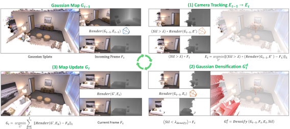
Figure 2. SplaTAM Overview。给定新 RGB-D frame，循环三步：(1) 用 silhouette-guided rendering 优化相机位姿；(2) 基于 silhouette + depth 残差加新 Gaussian；(3) 固定位姿，warm-start 上次 map 参数，用 keyframe set 更新 Gaussian。

Initialization

第一帧跳过 tracking（pose = identity），silhouette 全零 → 所有像素都用于初始化新 Gaussian：center 在 unproject 的 3D 点，color 取像素 RGB，opacity 0.5，radius 设为投影回去恰好 1 像素：

Equation 5. Initial radius

$$r=\frac{D_{\text{GT}}}{f}$$

Step 1: Camera Tracking

• Constant-velocity 初始化 pose：$E_{t+1}=E_t+(E_t-E_{t-1})$（相机参数化为 translation + quaternion）
• Gradient-based 迭代更新 pose，Gaussian 参数 frozen，loss 只在 $S(\mathbf{p})>0.99$ 的可信像素上算：

$$L_t=\sum _{\mathbf{p}}(S(\mathbf{p})>0.99)\left(L_1\right(D(\mathbf{p}))+0.5\cdot L_1(C(\mathbf{p})\left)\right)$$

Depth L1 + 0.5× color L1（权重经验调出来；rebuttal 给出 range 分析）。Silhouette gating 是核心：新观测的区域 map 未覆盖，若直接算 loss 会污染 pose 梯度。L1 在缺失 GT depth 像素上取 0（处理真实数据集的深度空洞）。

Step 2: Gaussian Densification

定义 densification mask：

$$M(\mathbf{p})=(S(\mathbf{p})<0.5)+(D_{GT}(\mathbf{p})<D(\mathbf{p}))\cdot (L_1(D(\mathbf{p}))>50\cdot \text{MDE})$$

两类像素需要新 Gaussian：

• (a) Silhouette 不足（$S<0.5$，map 未覆盖）
• (b) 前方有被遮挡的新几何——GT depth < rendered depth（GT 更近）且深度误差 > 50× MDE（median depth error），说明当前 map 漏掉了前方挡住后面已有几何的结构

❓ 50×MDE 的阈值在 rebuttal 中作者承认是 “empirically by visualizing the densification mask” 调出来的 magic number。这种经验阈值在 cross-dataset 上的鲁棒性存疑——ScanNet++ / Replica 都是 benign indoor，未在工业、户外、动态场景验证。

新 Gaussian 初始化方式同 first-frame：center 在 unproject 点，opacity 0.5，radius = $D_{GT}/f$。

Step 3: Map Update

• Camera poses fixed，Gaussian 参数更新
• Warm-start 自上一轮 map（不从头训）
• Keyframe 选择：每 $n$ 帧存一个 keyframe，优化 $k$ 个：当前帧 + 最近 keyframe + $k-2$ 个与当前帧 frustum overlap 最大的历史 keyframe。Overlap 定义为 “当前帧深度图反投影后落入历史 keyframe frustum 的点数”
• Loss 同 tracking 但不用 silhouette mask（要全像素优化），额外加 SSIM RGB loss，cull 掉 opacity≈0 或过大的 Gaussian（沿用 [Kerbl et al. 2023]，但只是其 culling 的子集——不含 splitting）

❓ Rebuttal Q8：作者承认没做 BA（jointly 优化 pose + map），理由是当前 3DGS rasterizer 不支持 batched rasterization，多 pose 联合优化不可行。这是个工程限制而非方法局限——说明 SplaTAM 不是严格意义上的 dense BA SLAM，全局一致性完全靠 keyframe overlap 局部处理。

---

3. Experiments

3.1 Datasets & Protocol

四个 benchmark：

• Replica [Straub 2019]: 合成 indoor，标准 RGB-D SLAM benchmark，位移小、depth 干净
• TUM-RGBD [Sturm 2012]: 真实场景，老相机 → RGB 运动模糊 + depth 稀疏
• ScanNet [Dai 2017]: 真实 indoor，质量类似 TUM-RGBD
• ScanNet++ [Yeshwanth 2023]: 作者引入用于 NVS 评估——DSLR 高质量 + 独立的 novel-view 采集轨迹；但连续帧位移非常大（“about the same as a 30-frame gap on Replica”）

ATE RMSE 为 tracking 指标；PSNR/SSIM/LPIPS + Depth L1 为 rendering 指标。Baselines 数字（除 ScanNet++）直接取自 Point-SLAM 论文。报告 3 seeds 平均。

3.2 Camera Pose Estimation

Table 1（摘录）. ATE RMSE [cm] ↓，baselines 数字取自 Point-SLAM

Dataset	NICE-SLAM	ESLAM	Point-SLAM	SplaTAM
Replica Avg	1.06	0.63	0.52	0.36
TUM-RGBD Avg	15.87	—	8.92	5.48
Orig-ScanNet Avg	10.70	—	12.19	11.88
ScanNet++ S1+S2	—	—	fail	1.2

核心观察：

• Replica：−30% over Point-SLAM（0.52 → 0.36cm）
• TUM-RGBD：−39%（8.92 → 5.48cm），但ORB-SLAM2 feature-based 1.98cm 仍明显更好——sparse feature 在 motion-blur + 稀疏 depth 的老 camera 数据上更鲁棒
• Orig-ScanNet：与 Point-SLAM/NICE-SLAM 打平（10+cm 级别，dense volumetric 方法在低质量相机上都崩）
• ScanNet++：Point-SLAM 和 ORB-SLAM3 完全 fail（texture-less 让 ORB-SLAM3 反复重初始化），SplaTAM 独家成功——这是论文最强的定量证据

❓ “Up to 2×” 的 claim 是 best case（TUM-RGBD 近 2×）；准确一般化应该是 “consistently better on 3 of 4 benchmarks, fails gracefully where dense methods fail together”。

3.3 Rendering Quality

Table 2. Replica Train-View rendering（8 scenes avg）

Metric	Vox-Fusion	NICE-SLAM	Point-SLAM*	SplaTAM
PSNR ↑	24.41	24.42	35.17	34.11
SSIM ↑	0.80	0.81	0.98	0.97
LPIPS ↓	0.24	0.23	0.12	0.10

* Point-SLAM 用 GT depth 做 rendering（不 apples-to-apples）

作者自己承认 train-view rendering “is irrelevant because methods can simply overfit to these images”——所以引入 ScanNet++ 做 novel-view benchmark：

Table 3. ScanNet++ Novel-View + Train-View Rendering（S1 + S2 avg）

Metric	Point-SLAM	SplaTAM
Novel PSNR ↑	11.91	24.41
Novel SSIM ↑	0.28	0.88
Novel LPIPS ↓	0.68	0.24
Novel Depth L1 [cm] ↓	N/A (需 GT depth)	2.07
Train PSNR ↑	14.46	27.98

2× novel-view PSNR gap 的真正原因是：Point-SLAM 在 ScanNet++ 上 tracking 完全 fail → map 位姿全错 → novel-view 渲染崩溃。不是 rendering module 不好，而是 tracking 不住。

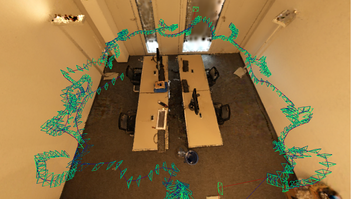
Figure 3. ScanNet++ S2 重建可视化：估计位姿（绿框 + 红轨迹）与 GT（蓝框 + 蓝轨迹）紧密贴合，稠密表面重建高保真。

Video. Replica Room 0 SplaTAM novel-view 渲染——直接从优化好的 Gaussian map 渲染 novel view RGB。作者明确披露同图比对中 NICE-SLAM / Point-SLAM 用了 GT novel-view depth，SplaTAM 不依赖。

Video. iPhone 在线重建 collage——RGB-D 来自 iPhone camera + ToF，展示真实手持设备可用性（源于 rebuttal 承诺）。

3.4 Ablations（Replica Room 0）

Table 4. Camera Tracking Ablation

Velo. Prop.	Silhouette Mask	Sil. Thresh.	ATE [cm] ↓	Dep L1 ↓	PSNR ↑
✗	✓	0.99	2.95	2.15	25.40
✓	✗	0.99	115.80	0.29	14.16
✓	✓	0.5	1.30	0.74	31.36
✓	✓	0.99	0.27	0.49	32.81

• Silhouette 是生死线：去掉后 ATE 从 0.27 → 115.80cm（tracking 彻底垮）
• Threshold 0.99 vs 0.5：5× 差距（1.30 → 0.27cm）——越严格 = 只在 well-optimized 像素算 loss，避免被新区域污染
• Velocity propagation 贡献约 11×（2.95 → 0.27cm）：对大位移场景尤其重要

Table 5. Color/Depth Loss Ablation

Track Color	Map Color	Track Depth	Map Depth	ATE [cm] ↓	Dep L1 ↓	PSNR ↑
✗	✗	✓	✓	86.03	fail	fail
✓	✓	✗	✗	1.38	12.58	31.30
✓	✓	✓	✓	0.27	0.49	32.81

• 只有 depth 不行：x-y 平面缺信息，tracking 完全崩
• 只有 color 能跑：但 ATE 5× 差、depth 恶化（但 densification 仍用 depth 做初始化）
• 两者协同才是 SOTA

Table 7 [Rebuttal]. Isotropic vs Anisotropic Gaussians on ScanNet++ S1

Distribution	ATE [cm] ↓	Train PSNR ↑	Novel PSNR ↑	Time [%] ↓	Memory [%] ↓
Anisotropic	0.55	28.11	23.98	100	100
Isotropic	0.57	27.82	23.99	83.3	57.5

结论：isotropic 在 SLAM 场景下几乎无损（ATE ±0.02cm、PSNR ±0.3 dB），换来 -17% time + -42% memory。支撑 §2.1 的 design 选择。

3.5 Runtime

Table 6. Runtime on Replica Room 0 (RTX 3080 Ti)

Method	Track/iter	Map/iter	Track/frame	Map/frame	ATE [cm]
NICE-SLAM	30 ms	166 ms	1.18 s	2.04 s	0.97
Point-SLAM	19 ms	30 ms	0.76 s	4.50 s	0.61
SplaTAM	25 ms	24 ms	1.00 s	1.44 s	0.27
SplaTAM-S	19 ms	22 ms	0.19 s	0.33 s	0.39

关键观察：

• SplaTAM 每 iter 渲染 1200×980 ≈ 1.2M 像素，Point-SLAM/NICE-SLAM 每 iter 只采 200-1000 像素——3 个数量级差距，但 rasterization 效率让 per-iter 时间相当
• SplaTAM-S 版本：tracking 40→10 iter/frame、mapping 60→15 iter/frame + 半分辨率 densification → 5× 加速，ATE 仅从 0.27 → 0.39cm 小幅降级。实用性强

3.6 Limitations

作者在 §5 末尾自己列出：

1. 对 motion blur、大 depth 噪声、激进 rotation 敏感（需 temporal modeling 缓解）
2. 未 scale 到大场景（建议走 OpenVDB 等 efficient 表示）
3. 依赖已知 camera intrinsics + dense depth（对比 monocular 的 Gaussian Splatting SLAM 工作，硬件门槛更高）

---

4. Concurrent Work

作者在 project page 罕见地诚实列出 5 篇同期 3DGS-SLAM 工作，思路各异：

• GS-SLAM：coarse-to-fine tracking + sparse Gaussian selection
• Gaussian Splatting SLAM (MonoGS)：monocular（无需深度），densification 用 depth 统计
• Photo-SLAM：ORB-SLAM3 tracking + 3DGS mapping 解耦
• COLMAP-Free 3DGS：mono depth estimation + 3DGS
• Gaussian-SLAM：DROID-SLAM tracking + 主动/非主动 3DGS sub-maps

这种 cluster 本身是个信号——3DGS 出来 5 个月内 5 组独立收敛到 “用它做 SLAM”，说明显式可微表示对 SLAM 是 “obvious next step”。SplaTAM 的差异化在 silhouette-guided unified pipeline（三步全用同一 differentiable rasterizer，没有 hybrid tracker），而非 Photo-SLAM/Gaussian-SLAM 的 hybrid 耦合。

---

关联工作

基于

• 3D Gaussian Splatting [Kerbl et al. SIGGRAPH 2023]: 底层表示与可微 rasterizer
• Dynamic 3D Gaussians [Luiten et al. 2023]: 同一作者前作，把 3DGS 扩到 dynamic scene 的 6-DOF tracking——SplaTAM 是其 SLAM 化

对比 (Implicit SLAM baselines)

• iMAP [Sucar et al. ICCV 2021]: 第一个用 neural implicit 做 SLAM 的工作
• NICE-SLAM [Zhu et al. CVPR 2022]: hierarchical multi-feature grids，扩展 iMAP scalability
• Point-SLAM [Sandström et al. ICCV 2023]: neural point cloud + volumetric rendering，最强 implicit baseline——SplaTAM 正面对比对象
• ESLAM [Johari et al. CVPR 2023]: hybrid SDF-based
• Vox-Fusion [Yang et al. 2022]

对比 (Traditional dense SLAM)

• KinectFusion [Newcombe 2011]: TSDF 经典
• BundleFusion [Dai 2017]: globally consistent TSDF
• ElasticFusion [Whelan 2015]: surfel-based，differentiable rasterization 先驱
• BAD SLAM [Schops 2019]: bundle-adjusted RGB-D direct method
• ORB-SLAM2/3 [Mur-Artal, Campos]: feature-based sparse，TUM-RGBD 仍 SOTA

Concurrent (3DGS-SLAM)

• GS-SLAM, Gaussian Splatting SLAM (MonoGS), Photo-SLAM, COLMAP-Free 3DGS, Gaussian-SLAM——见 §4

数据集

• ScanNet++ [Yeshwanth ICCV 2023]: 高保真 indoor benchmark，作者引入用于 NVS evaluation

---

论文点评

Strengths

1. 方法极简而 unified：tracking / densification / map update 共用一套 differentiable splatting + photometric loss，没有 ORB-SLAM / DROID 这样的外部 tracker。silhouette mask 一个机制同时解决 tracking gating 和 densification 触发——是 “simple, scalable, generalizable” 的好例子（Ablation Table 4 验证：去掉 silhouette 直接 tracking 崩）
2. Direct gradient 论证有 first-principles 味道：作者明确指出 “Gaussian 参数到像素是近线性投影 + camera 等价于 inverse scene motion”，这是为什么 implicit-SLAM tracking 慢/难收敛的根本原因。这种 framing 比单纯 benchmark 数字更有 explanatory power
3. Honest disclosure：concurrent work 全列；rebuttal 中承认 50×MDE 是经验值；明确披露 NICE-SLAM/Point-SLAM 在 NVS 时使用 GT depth，SplaTAM 不依赖；ATE Orig-ScanNet 没赢也照实写 “competitive”。这种诚实度在 SOTA-claiming 论文里罕见
4. 完整 ablation 覆盖设计关键点：silhouette threshold、velocity propagation、color-only vs depth-only 都独立验证；rebuttal 补齐 isotropic vs anisotropic
5. Open source + iPhone demo：codebase + 真实手持设备（camera+ToF）验证，易于复用。SplaTAM-S 变体提供 5× 加速/小幅 ATE 降级的实用选项

Weaknesses

1. 依赖准确 RGB-D：硬件门槛较高。Concurrent 的 Gaussian Splatting SLAM（MonoGS）直接做 monocular，方法上 ceiling 更高——SplaTAM 的 first-principles 优势部分被硬件依赖稀释
2. No loop closure / global BA：纯前向增量 + 局部 keyframe overlap，silhouette gating 是局部机制。Rebuttal Q8 作者承认 “BA doesn’t help” 但归因于 rasterizer 不支持 batched——是工程限制不是方法极限。大场景长轨迹下 drift 必然累积，论文未讨论
3. Magic numbers 较多：$S>0.99$（tracking）、$S<0.5$（densification）、$50\times \text{MDE}$、opacity $0.5$ init、color-loss weight $0.5$——这些阈值在 Replica/ScanNet++ 这类 benign indoor 之外的鲁棒性未充分验证
4. Limitations 开诚布公但未解决：motion blur + 激进 rotation + 大场景——都是 embodied / AR 实际落地必须应对的场景。论文定位为 “opens up avenues”
5. Tracking 是 per-frame iterative optimization：每帧 40 iter（SplaTAM-S 10 iter），“online” 但不是严格 real-time（Replica 1 s/frame）。对 camera 10+ FPS 输入的实时处理尚不够

可信评估

Artifact 可获取性

• 代码: 完整开源（inference + training），github.com/spla-tam/SplaTAM；README 附 Replica / ScanNet / ScanNet++ / TUM-RGBD / iPhone 的独立 config
• 模型权重: N/A —— SLAM 是 per-scene online optimization，无 pretrained weights
• 训练细节: README 提供完整超参 config（每 dataset 独立 YAML 含 tracking/mapping iter 数、loss 权重、threshold）
• 数据集: 全部公开 benchmark（Replica / TUM-RGBD / ScanNet / ScanNet++）

Claim 可验证性

• ✅ 400 FPS rendering @ 876×584：可由开源代码 + 单 GPU 验证；splatting rasterization 速度有 [Kerbl 2023] 上游证据
• ✅ 优于 NICE-SLAM / Point-SLAM 的 ATE RMSE：开源 + 标准 benchmark 可独立复现；作者注明 baselines 数字直接取自 Point-SLAM
• ✅ Ablation 是干净的 component-wise (Table 4, 5, 7)：逐项移除设计选择，结论 grounded
• ⚠️ “Up to 2× SOTA”：best-case 数字（TUM-RGBD 近 2×、novel-view PSNR > 2×）；Orig-ScanNet 仅 “competitive”。一般化应说 “consistently better on 3 of 4 benchmarks”
• ⚠️ NVS 对比 Point-SLAM 的 12.47 PSNR gap：主因 Point-SLAM tracking 失败而非 rendering 本身弱——apples-to-oranges 风险；Fair 对比应是 “post-hoc align poses 后 rendering 质量”
• ⚠️ Sub-cm tracking on texture-less：Fig 1 的 “baselines fail” 是定性 cherry-pick，未量化 failure rate（如多少序列/百分比下 ORB-SLAM3 触发 re-init）

Notes

• 对我研究的意义：3DGS-SLAM 这一 line 与 spatial intelligence / embodied perception 间接相关——若 embodied agent 需要 online 构建 high-fidelity 可查询 3D map，SplaTAM 这类方法是自然候选。但纯 SLAM 不是我研究主线，本笔记定位为 indexed reference
• 可借鉴的 design pattern：silhouette mask 作为 epistemic uncertainty proxy 是个简洁 idea——“用 model 自身的覆盖度判断该不该相信 loss”。在其他在线学习 / 增量优化场景也许可借鉴（如 streaming VLM continual learning 中用 “model confidence” 做 sample gating）
• Pivot 信号：5 篇并发 = obvious idea。“早一步发出来” 的 SplaTAM 拿到 CVPR + 高引，但同期任一篇都能做出类似贡献。从 idea-generation 角度：当方法变成 obvious 时，再追随就是 marginal contribution——真正的 edge 在更难的问题（mono？loop closure？dynamic？）
• Open questions：
  • 3DGS-SLAM 后续是否解决了 loop closure / global BA？需要查 2024-2025 follow-up（LoopSplat 等）
  • Isotropic 假设在反光 / 细结构 / 户外场景是否仍成立？rebuttal 只给了 indoor ScanNet++
  • 简化掉 SH 对 high-variance lighting 的影响？

Rating

Metrics (as of 2026-04-24): citation=574, influential=128 (22.3%), velocity=20.07/mo; HF upvotes=2; github 2101⭐ / forks=236 / 90d commits=0 / pushed 673d ago · stale

分数：2 - Frontier
理由：SplaTAM 是 CVPR 2024 早期 3DGS-SLAM 代表作——开源完整、被 GS-SLAM/MonoGS/Photo-SLAM 等后续 3DGS-SLAM 普遍作为 baseline；silhouette-guided unified pipeline + direct-gradient 论证具备 first-principles 清晰度（Strengths 1-2）；消融与 runtime 完整（Table 4-7）。不给 3 的原因是按 field-centric rubric——SLAM 不是我的主线方向（VLA / Agent / Embodied），且在 3DGS-SLAM 内部同期并发 5 篇思路收敛（§4），SplaTAM 是时间上稍先的 Frontier 而非独家奠基；不给 1 的原因是它仍是当前 3DGS-SLAM 方向的标准对比对象，作为 indexed reference 对 embodied spatial mapping 的延伸阅读仍具价值。